5. Analysis and Diagnostics

5.1 Debug Compare Existing Studies

Purpose

This chapter explains how to compare a running study with one or more existing studies during a debug run.

Before you start

• The current study is paused in Debug mode.

• You have DV/SV files or study outputs from one or more existing alternatives.

Procedure

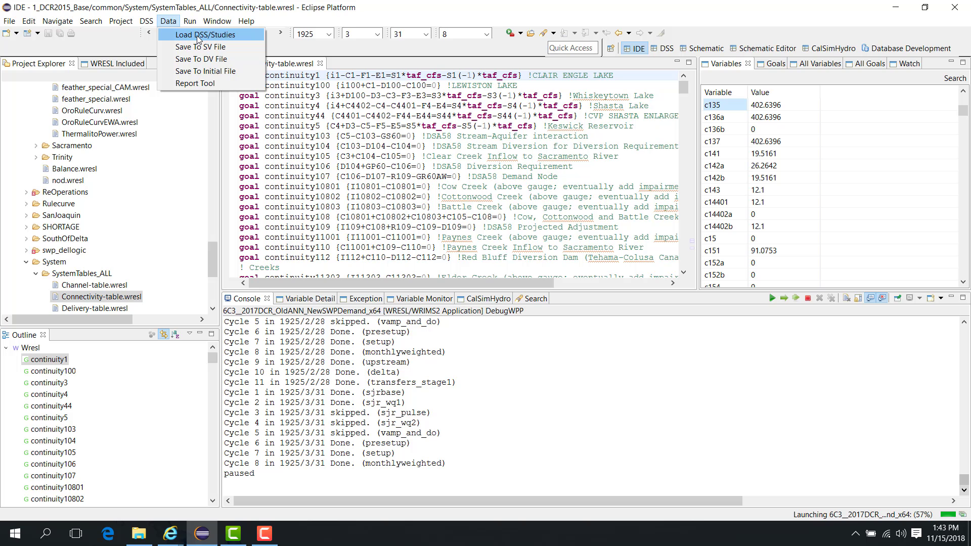
Pause the model in Debug mode at a point of interest, such as March 31, 1925.

To compare the current run with an existing study:

1. Open the Data menu.

2. Choose Load DSS or Study.

WRIMS 3 GUI allows up to eight alternatives:

• Alternative 1–4 load DV and SV files from existing studies.

• Alternative 5–8 load intermediate LP (ILP) files.

This chapter focuses on Alternative 1–4.

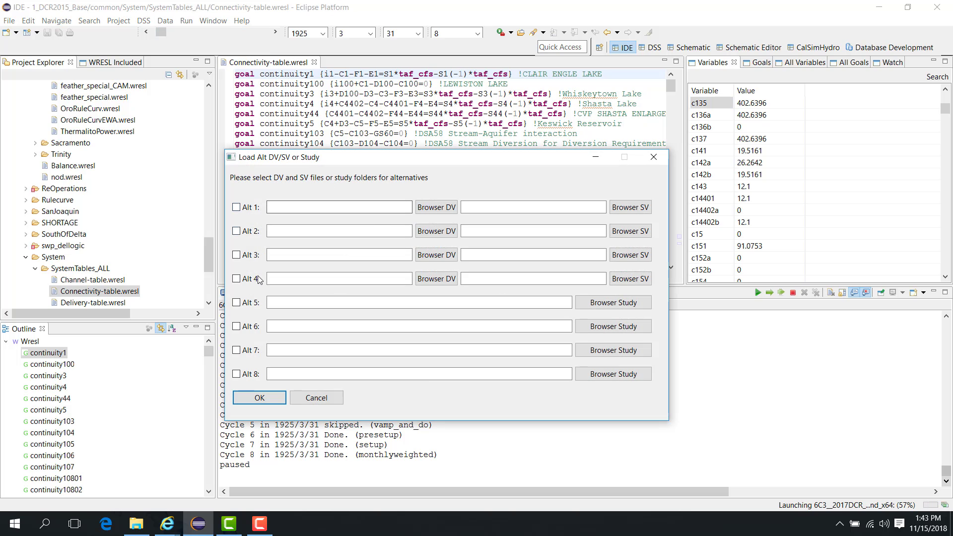
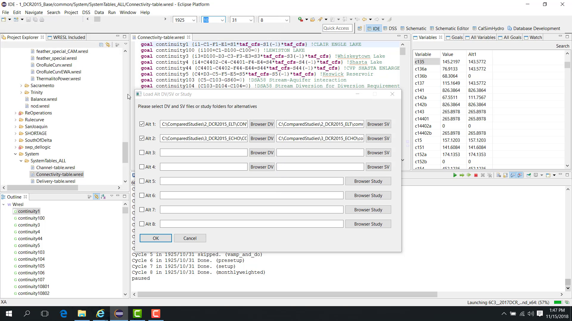
Load an alternative study

To load Alternative 1, browse to the existing study and select the DV and SV files.

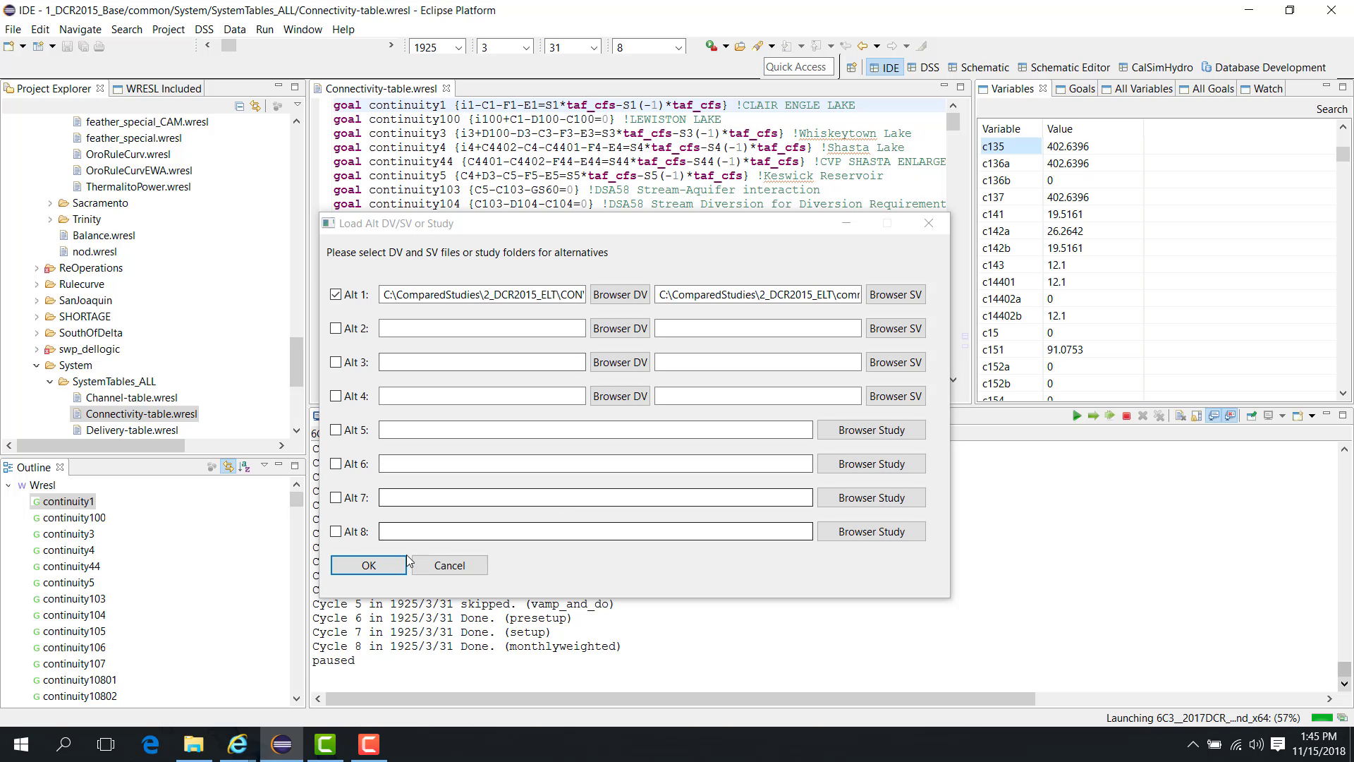
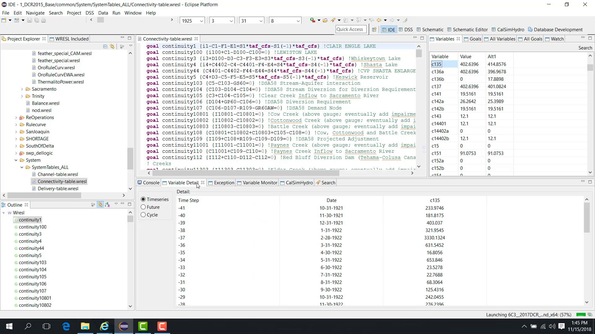
After loading:

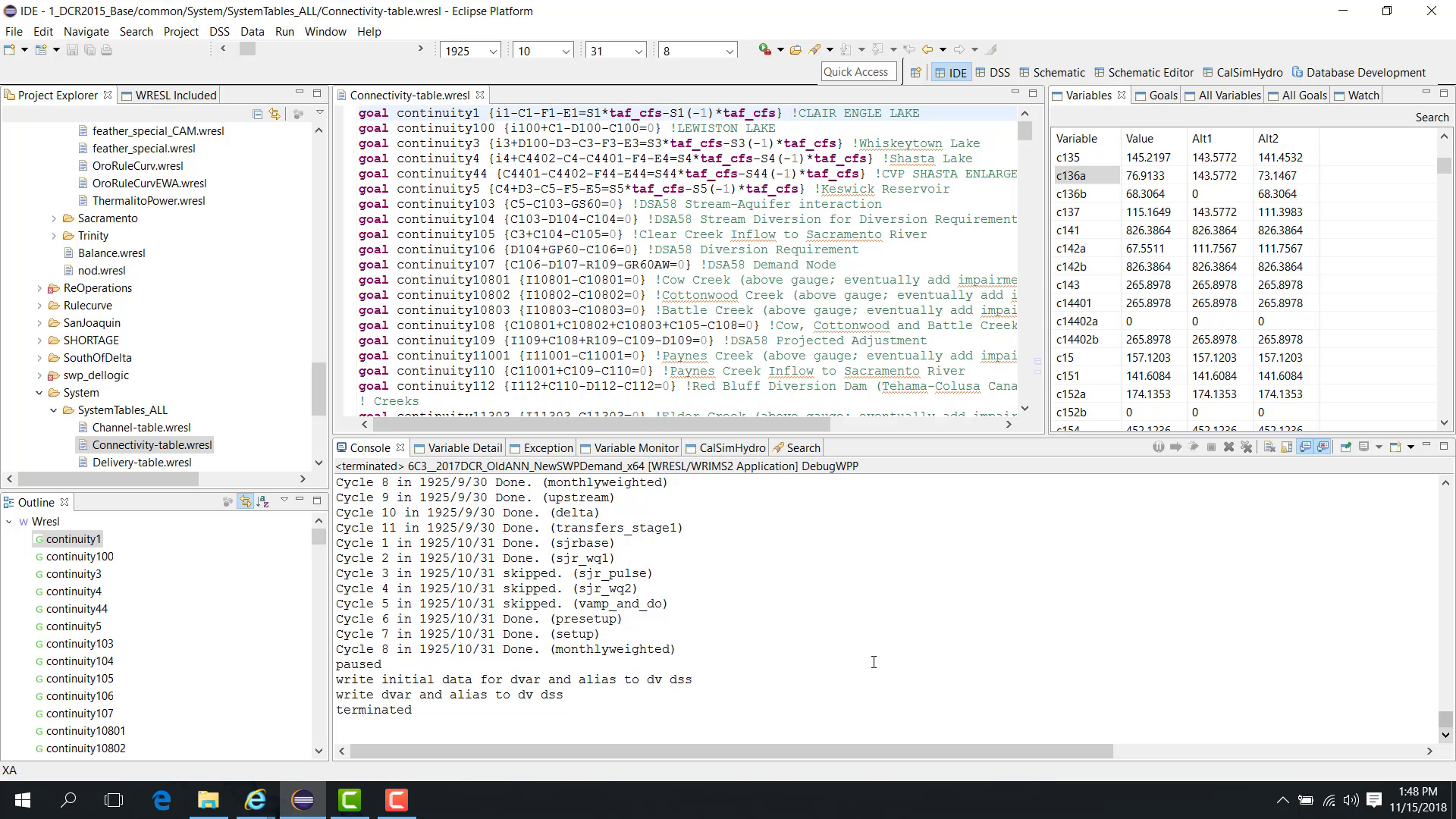
• variables show values for the current run;

• variables also show values for Alternative 1.

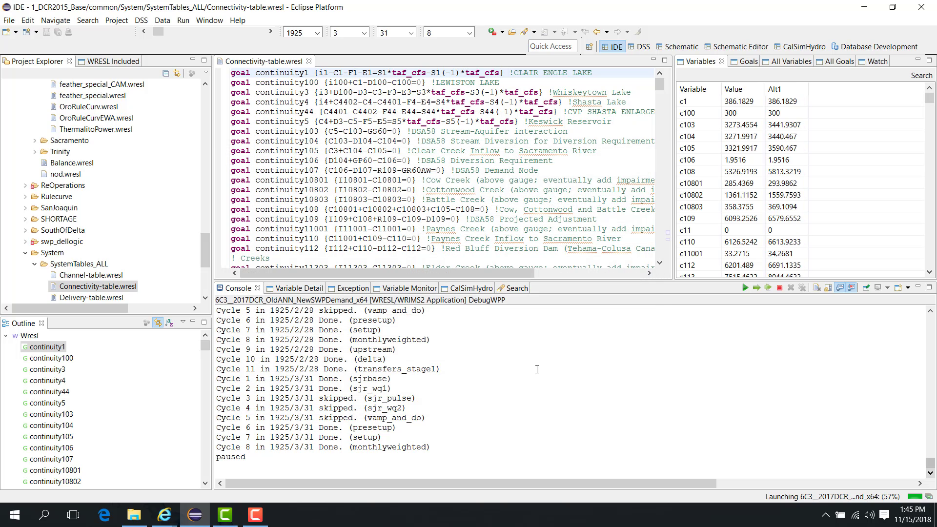
If you click a variable, the Variable Detail panel shows both the current-run value and the alternative value.

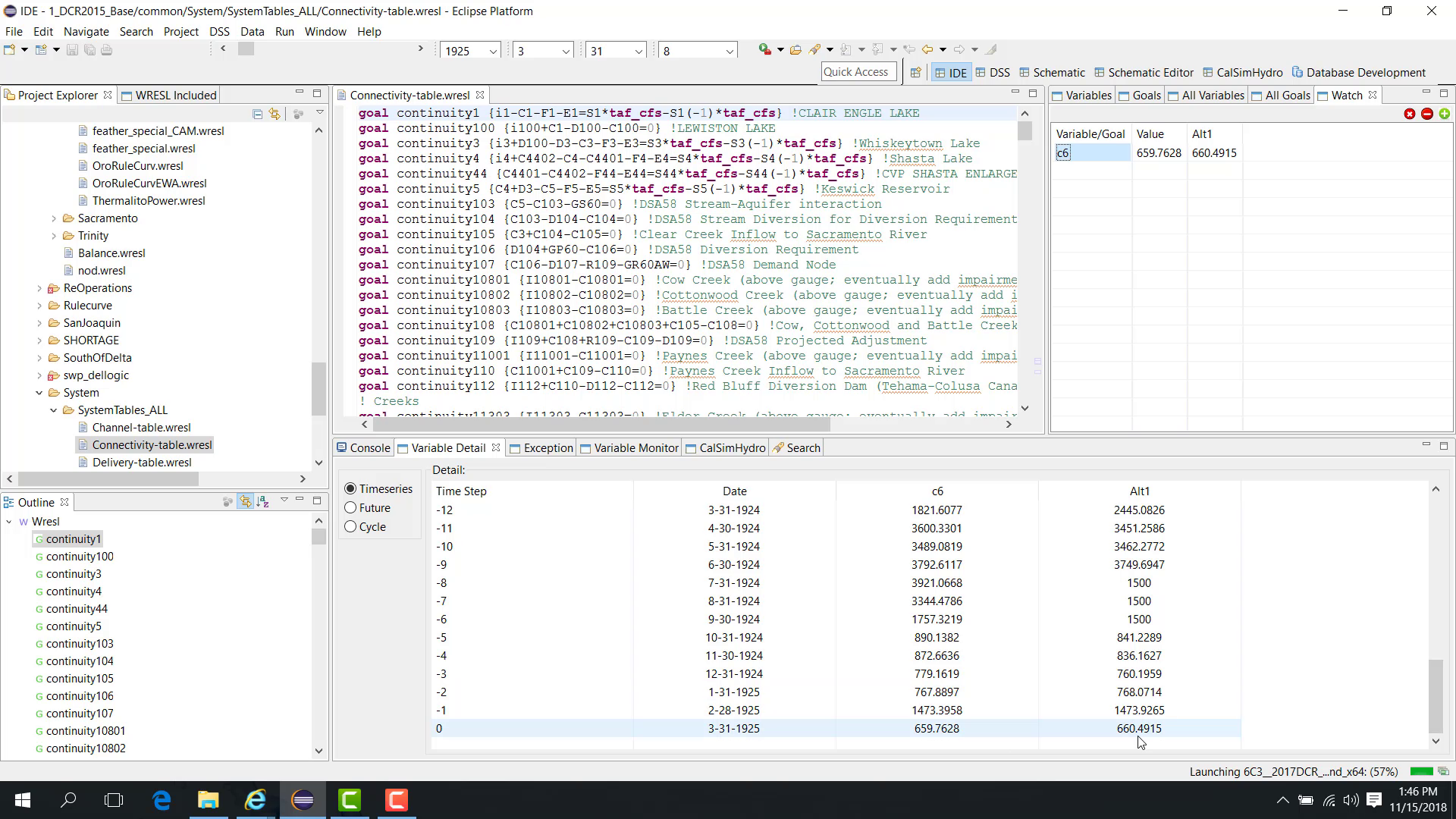
Compare watched variables

The Watch panel can also be used to compare watched variables between the current run and the alternative.

A watched variable such as C8 or C6 can display both current-run and alternative values through time.

Continue the run

When the run resumes and moves to a later time step, the comparison values update accordingly.

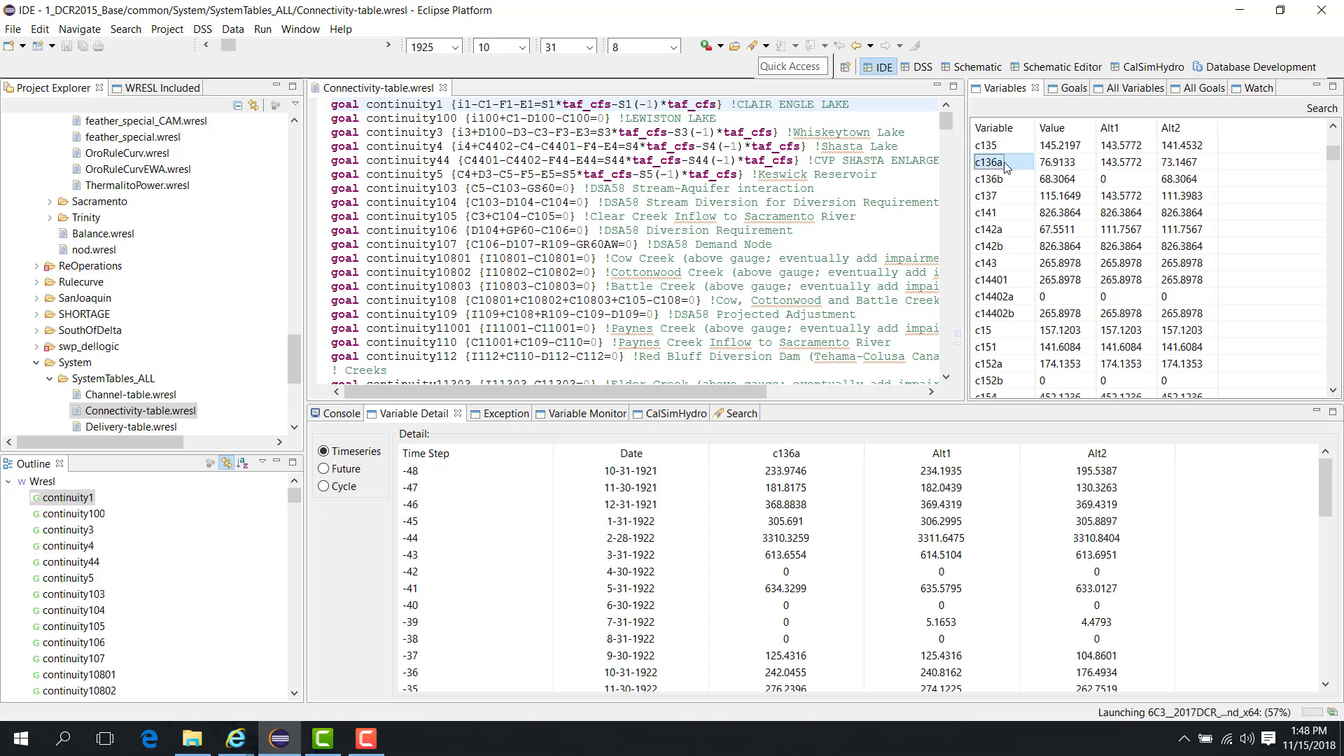
Load another alternative

Load Alternative 2 in the same way.

At that point, the interface can compare:

• the current run;

• Alternative 1;

• Alternative 2.

When a variable is selected, the Variable Detail panel shows all loaded comparison values.

If the study is terminated before completion, the current run is still saved to DSS.

Notes

• Alternatives 1–4 are used for existing study DV/SV comparisons.

• This workflow is useful for regression checking, troubleshooting, and understanding why a current run diverges from a known baseline.

Related sections

• 2.5 Basic Perspectives

• 7.1 Special Batch Run GUI

• 8.1 DSS Wrims DSS Perspective

5.2 Debug Filter Goals

Purpose

This chapter is easier to understand after you are comfortable with paused inspection, watched variables, and goal views. See 09. Debug Pause Variable Goal View and 12. Debug Watch Variables Goals as preparation.

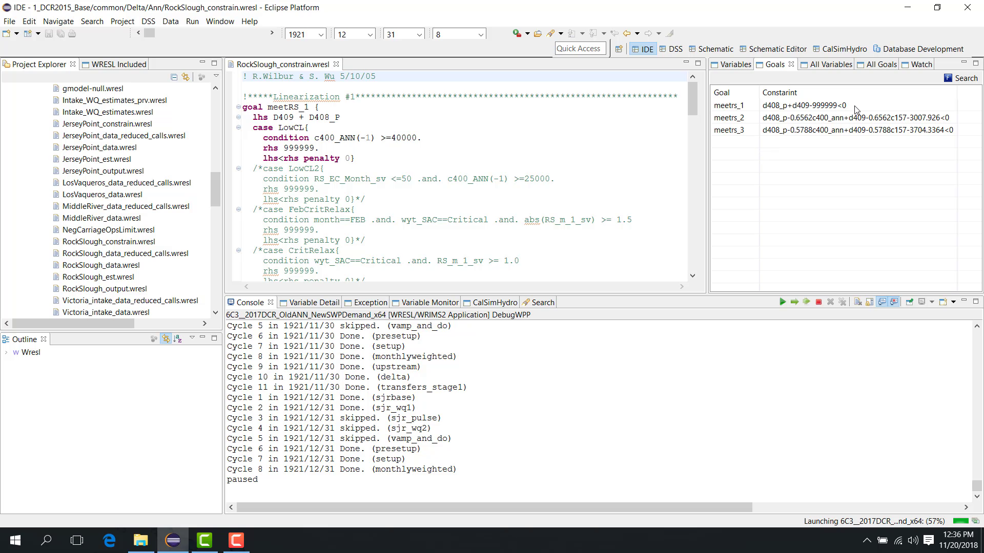
This chapter shows how to use a filtering file to evaluate selected goals and determine whether they should be treated as controlling goals.

Before you start

• The study is paused in Debug mode.

• You have a goal-filter file with goal names, aliases, and optional tolerances.

Procedure

For the controlling-goal concept and tolerance behavior, see 2.4 Controlling Goals and Goal Tolerance.

A filtering file provides another way to evaluate controlling goals.

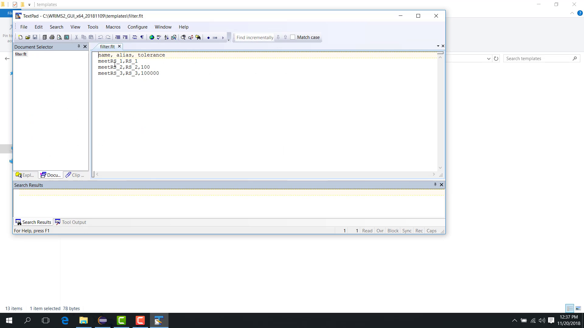
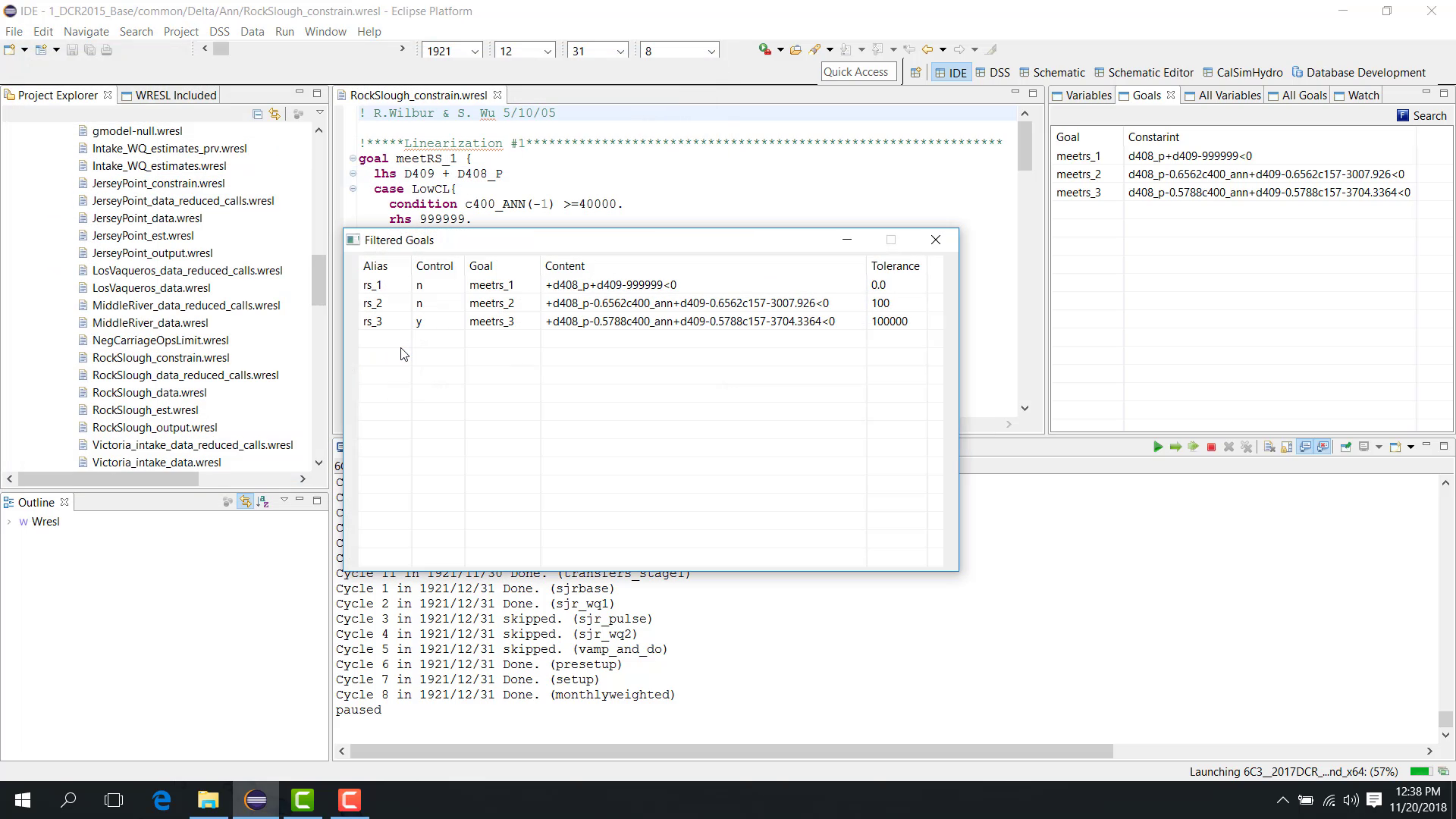
A sample filtering file contains:

• the goal name;

• an alias;

• a tolerance.

The tolerance rules are described in 2.4 Controlling Goals and Goal Tolerance.

For example, a tolerance of 100 means the goal is treated as controlling if the difference is less than 100.

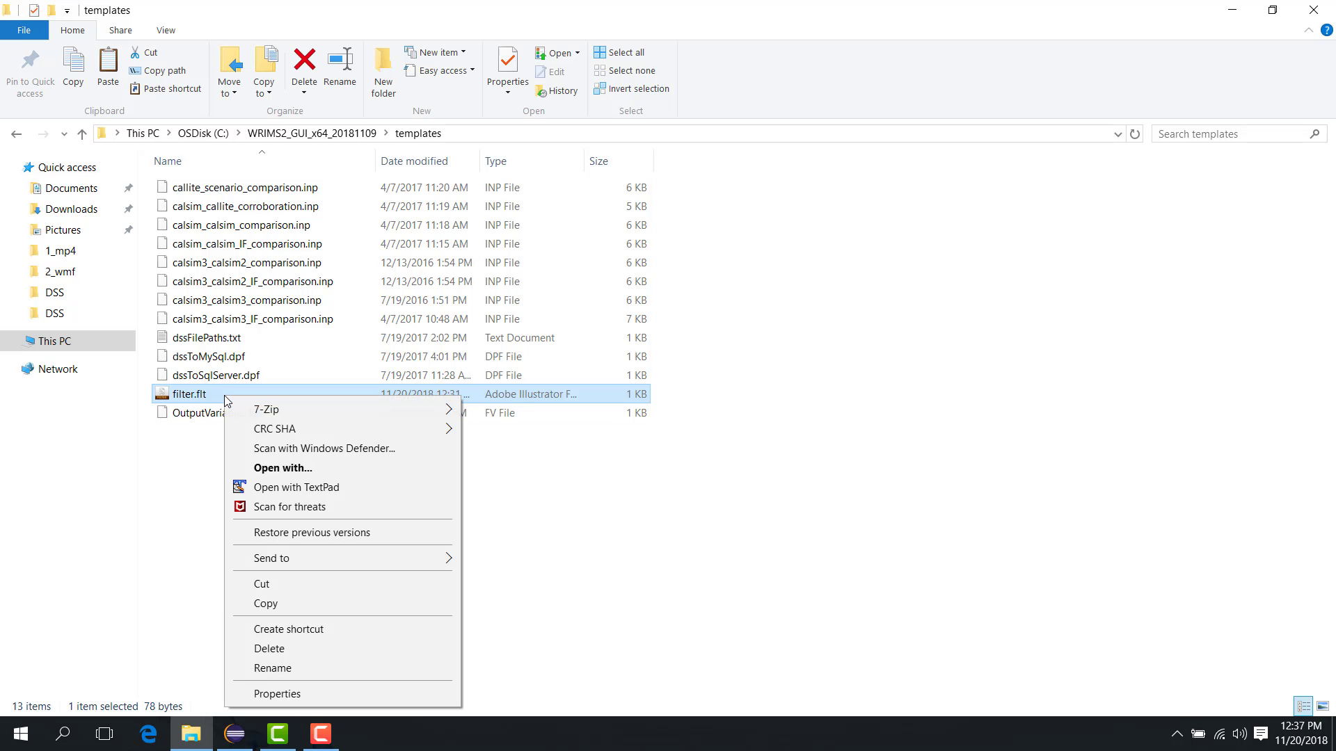
To use the filter file:

1. Click the Filter Goals button.

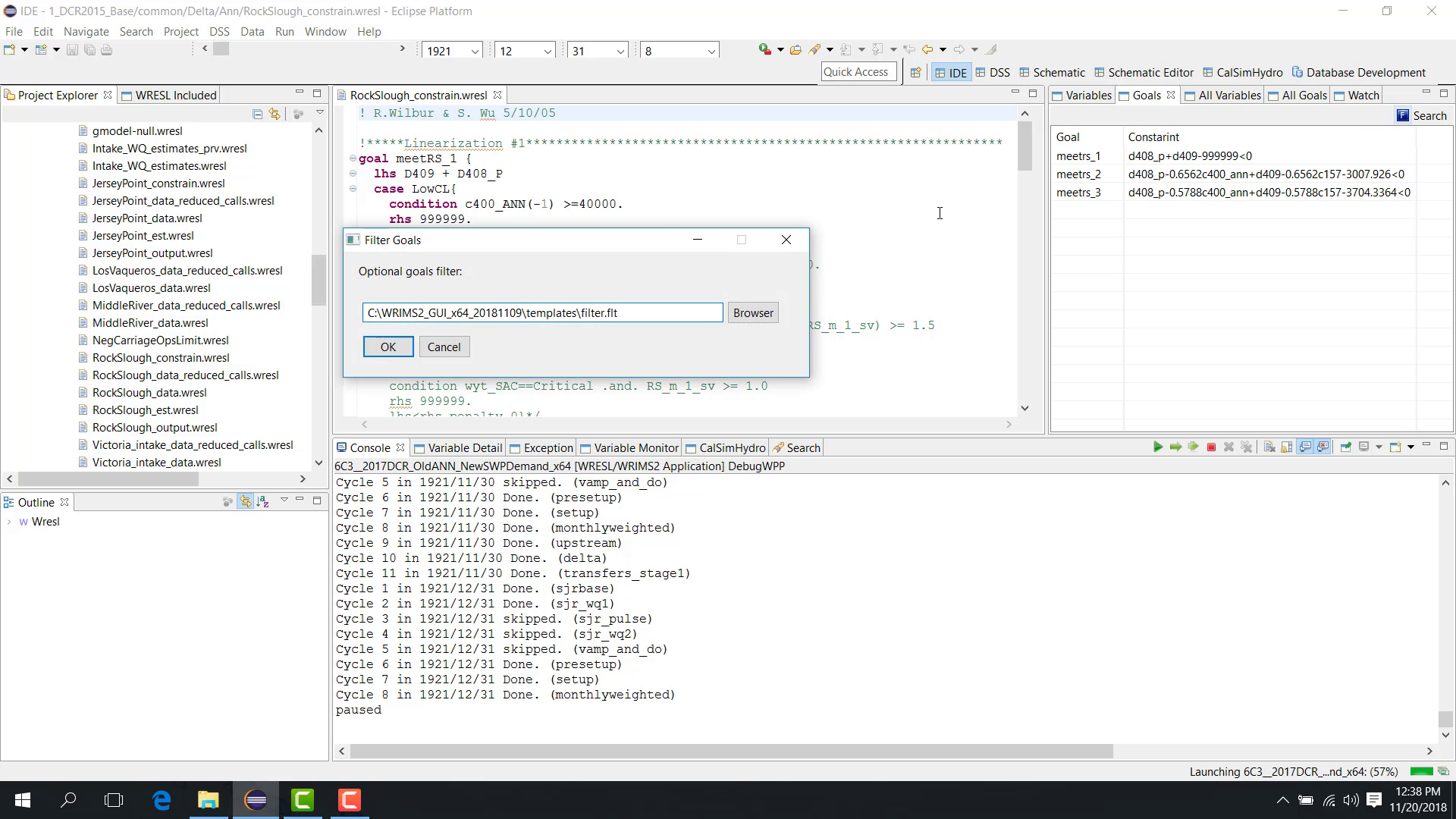
2. Browse to the filter file.

3. Click OK.

WRIMS 3 GUI displays a dialog with the filtered goals and indicates which of them are controlling under the specified tolerance.

A very large tolerance may be useful for demonstration, but it is not typical for production analysis.

Notes

• A tolerance allows a goal to be treated as controlling even when the left-hand side and right-hand side are not exactly equal.

• Use realistic tolerances for analysis; very large tolerances are usually for demonstration only.

Related sections

• 4.1 Debug Pause Variable Goal View

• 4.4 Debug Watch Variables Goals

• 5.3 Debug Force Variable Resimulation

5.3 Debug Force Variable Resimulation

Purpose

This chapter builds on earlier debugging concepts, especially paused execution, goal inspection, and filtered analysis. Review 09. Debug Pause Variable Goal View and 21. Debug Filter Goals if needed.

This chapter shows how to force a variable to a specified value and re-simulate the current time step to analyze objective-function impact.

Before you start

• The study is paused at the time step and cycle you want to investigate.

• You know the variable and trial value you want to force.

Procedure

Pause the model in Debug mode at a selected time step and cycle, such as:

• December 1921;

• cycle 10.

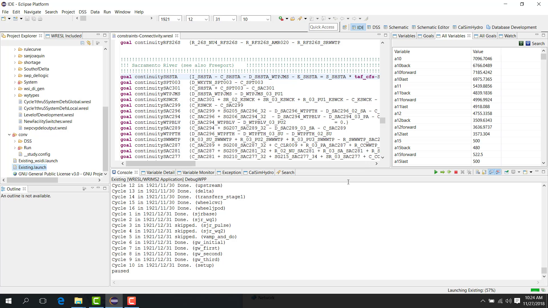
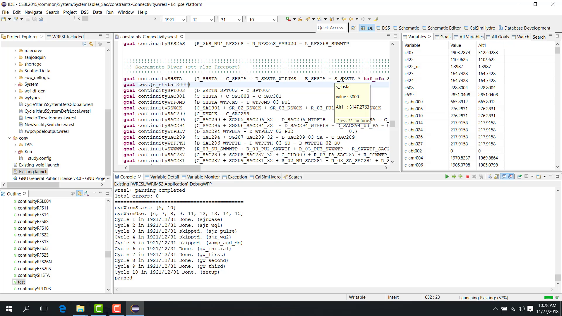
In the example shown here, the current value of s_shsta is 3147.

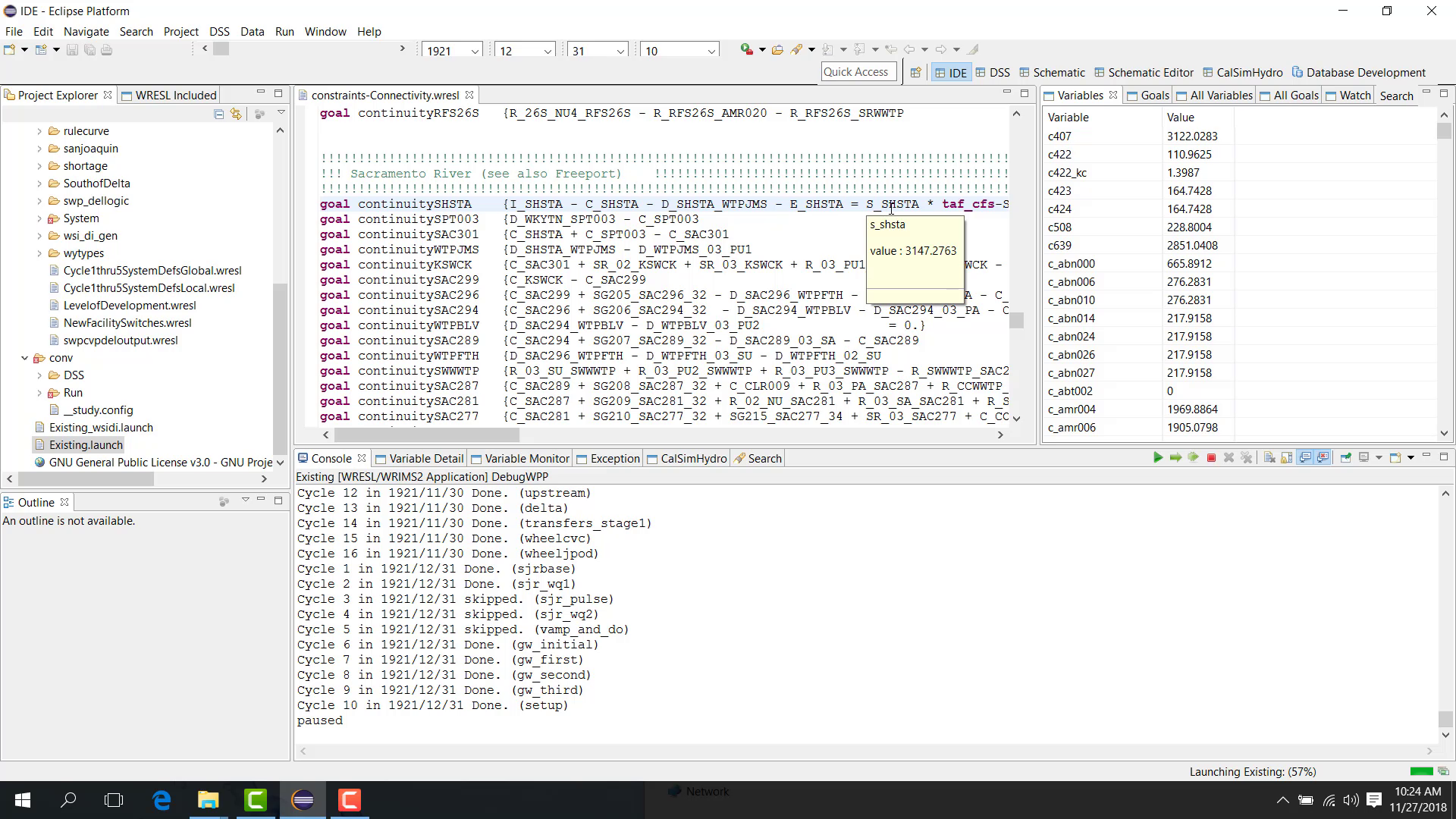
The objective is to test what happens if s_shsta is forced to 3000.

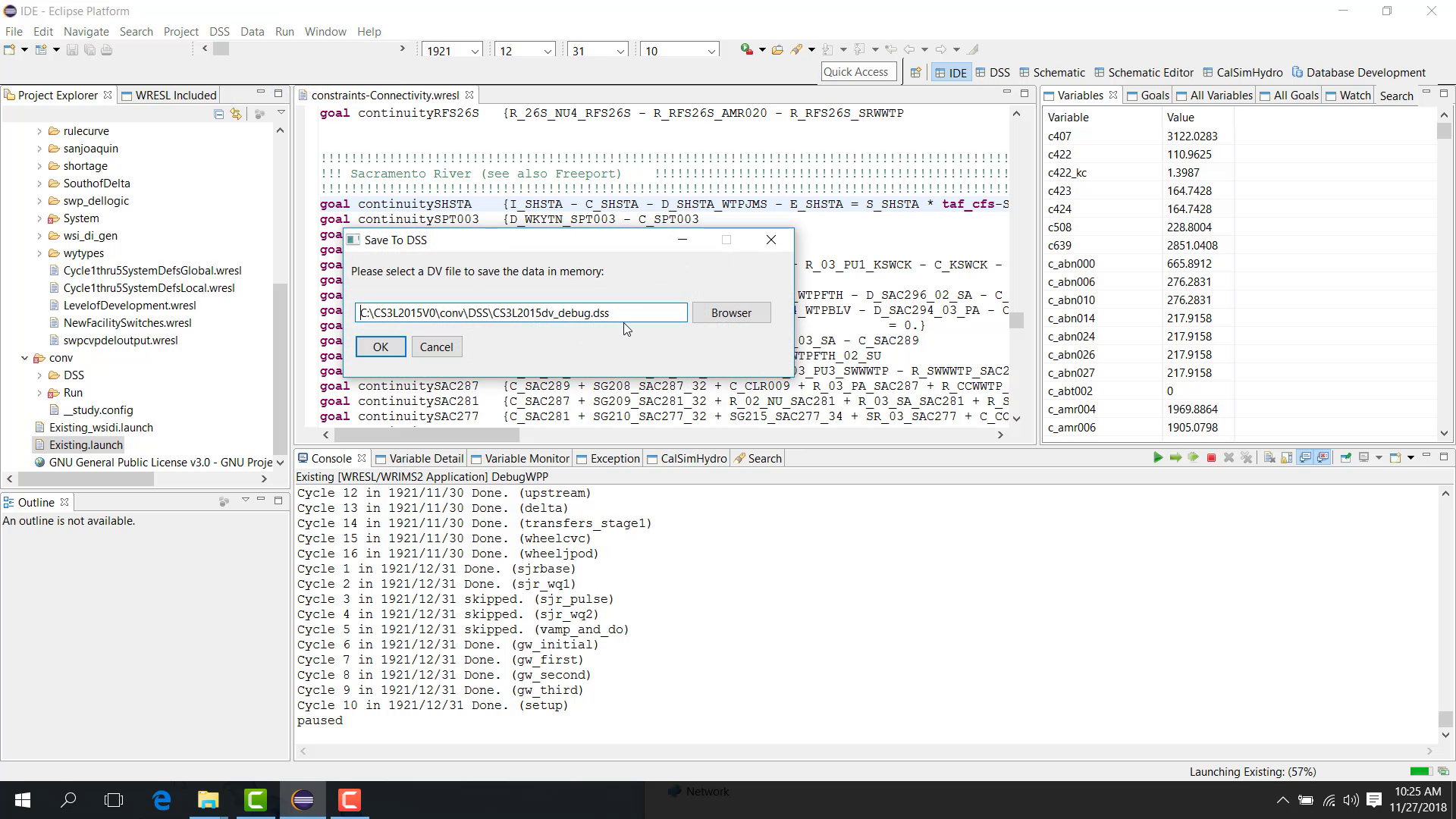
Step 1: Save the current DV results

First, save the current results to the DV file.

Step 2: Load the saved DV file as Alternative 1

Load the saved DV file as Alternative 1 so that the original value is available for comparison.

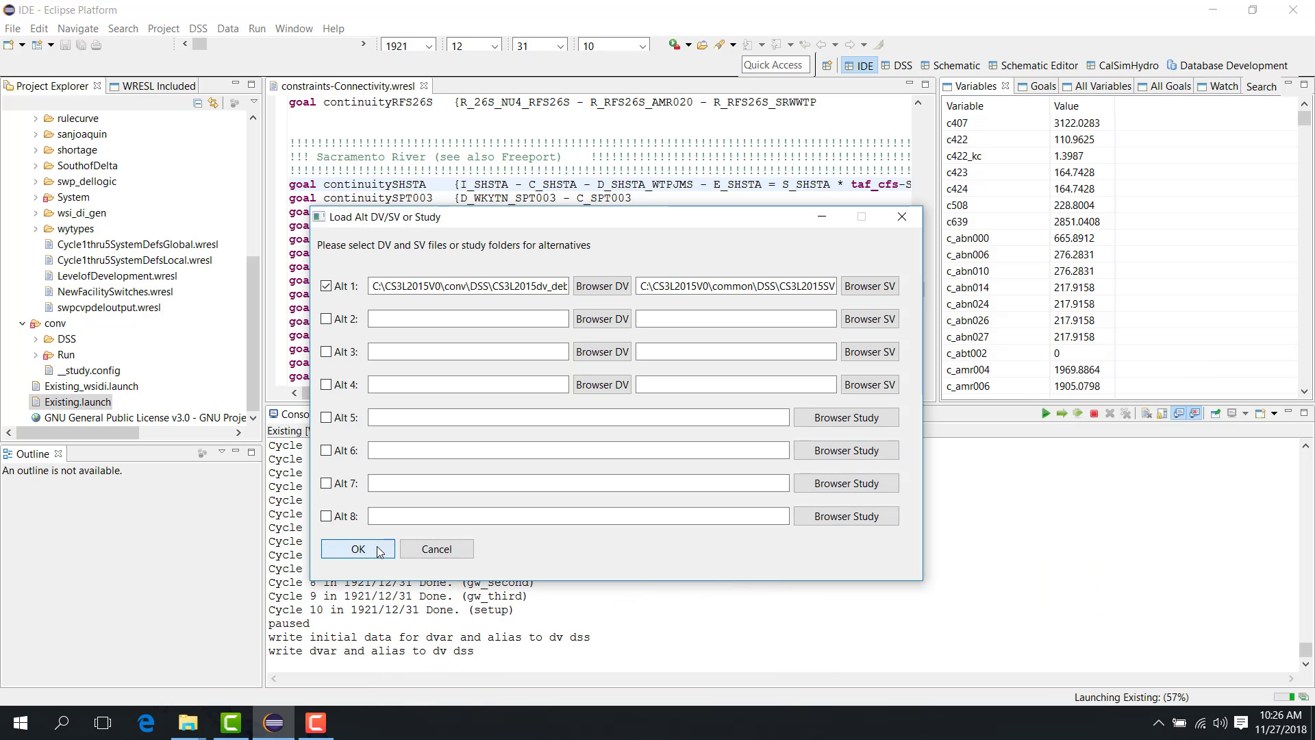
At this point:

• current run = original value;

• Alternative 1 = same original value.

Step 3: Add a forcing goal

Add a new goal to the WRESL code, using a unique name so that it does not conflict with any existing goal.

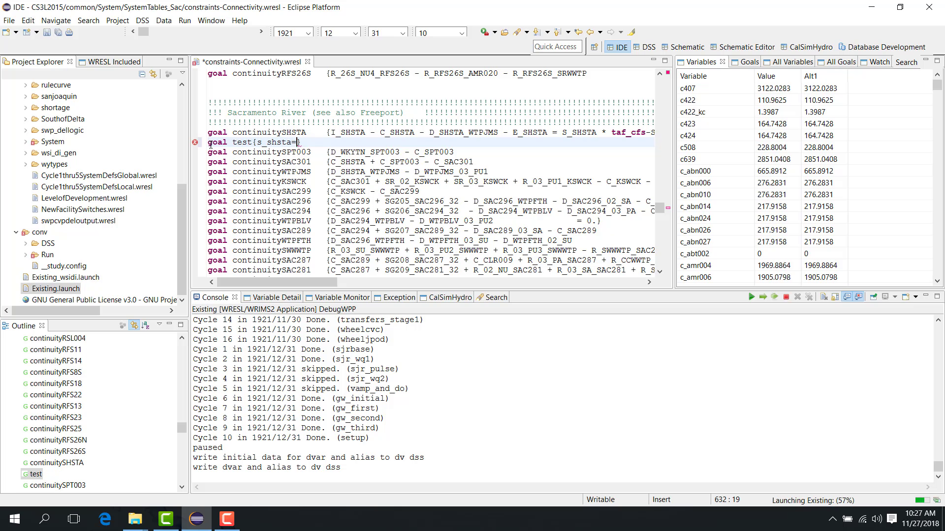
A forcing goal can be written as:

goal test { s_shsta = 3000 }

Save the file after adding the new goal.

Step 4: Re-simulate

To rerun the time step with the new forcing goal:

1. Open Run > Re-simulate.

2. Select the current time step.

3. Enable Re-compile WRESL Code because the WRESL source has changed.

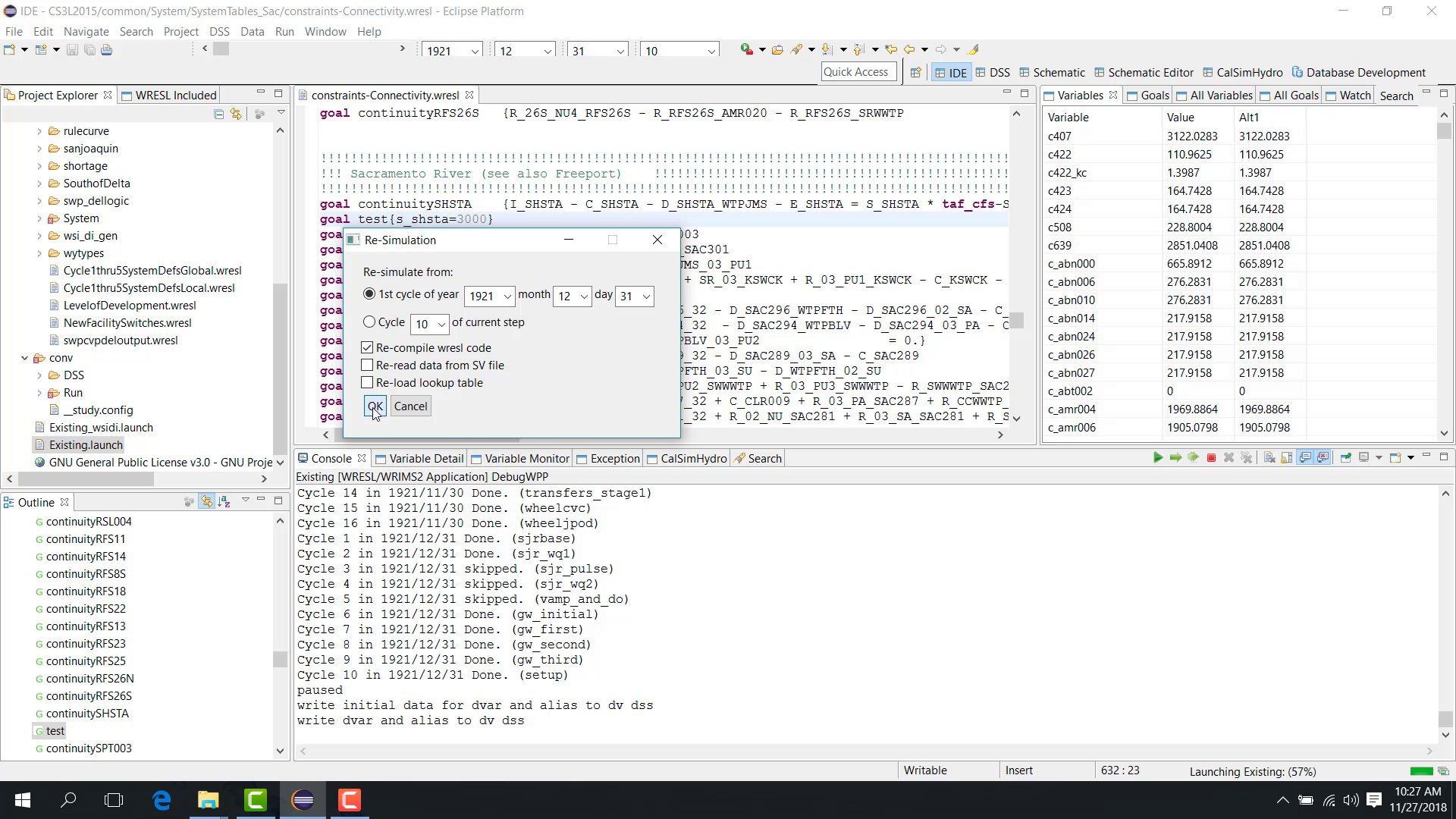
4. Click OK.

The time step is rerun using the new goal.

At this point:

• current run = forced value, such as 3000;

• Alternative 1 = original value, such as 3147.

Step 5: Analyze the objective function

To analyze the objective-function impact:

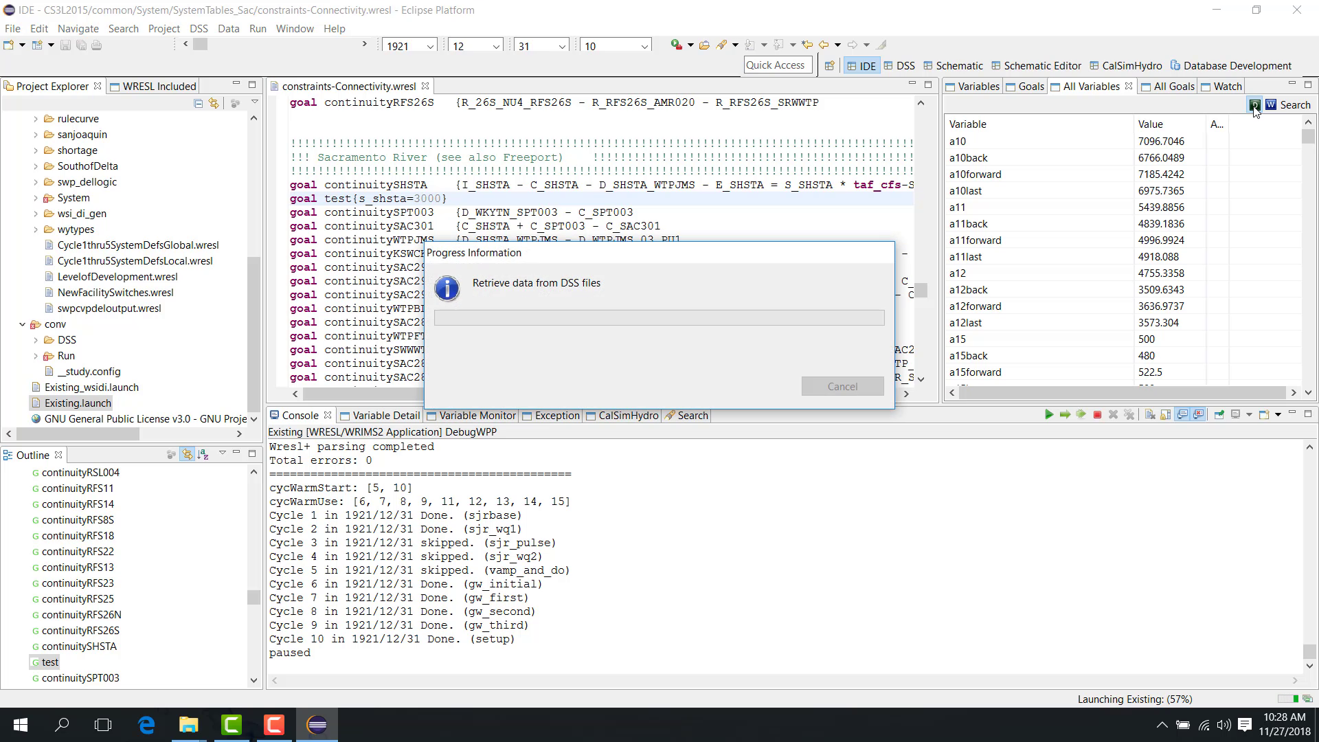
1. Open All Variable.

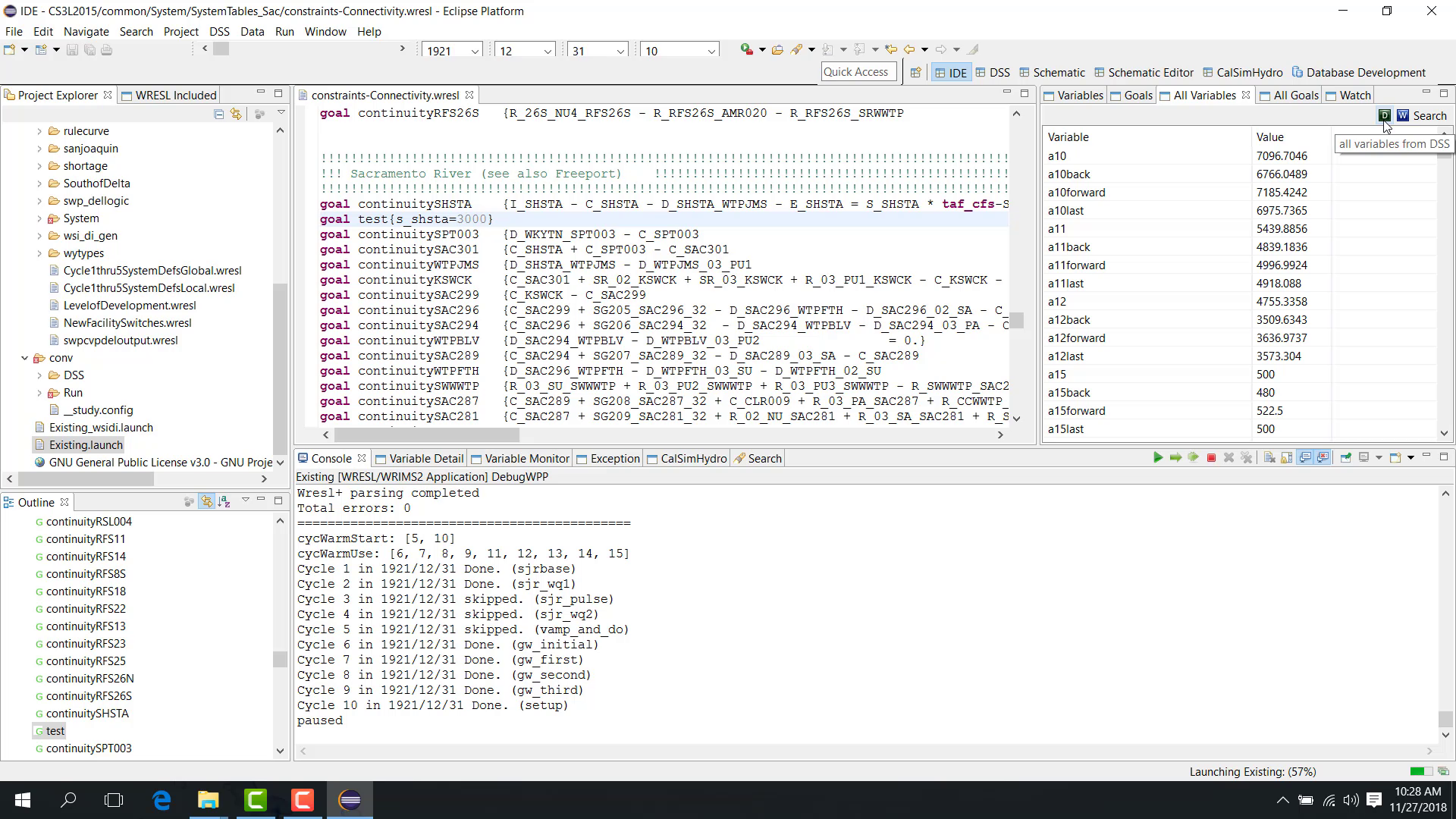
2. Retrieve the alternative data.

3. Open Weighted Variable.

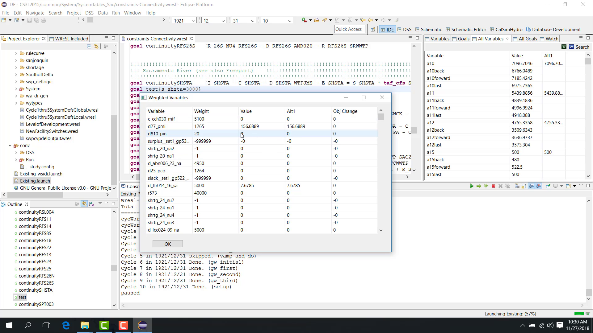
4. Compare the current run and Alternative 1.

5. Sort by objective change.

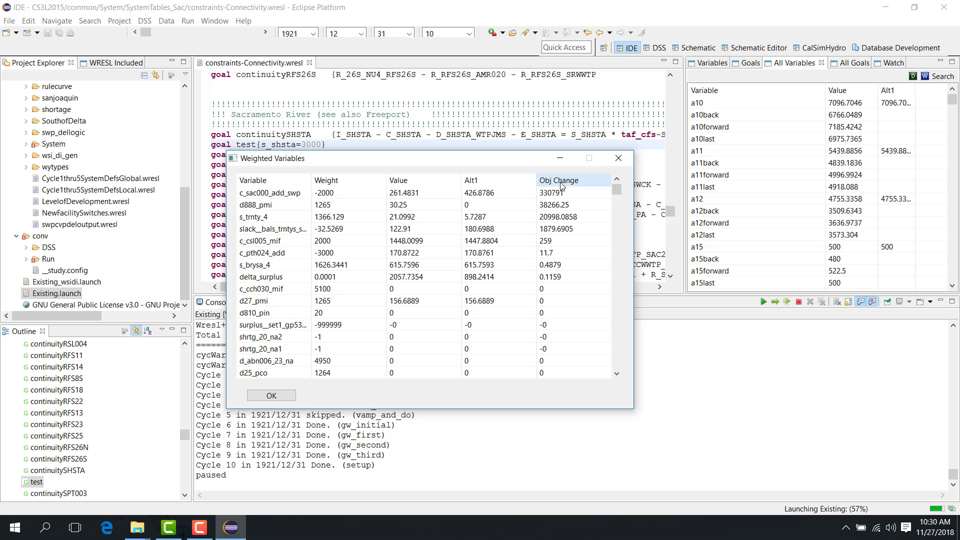
This comparison shows:

• which variables increase the objective;

• which variables decrease the objective;

• which changes contribute most to the overall difference.

Notes

• Save the current DV result first so that the forced rerun can be compared against the original case.

• Recompile WRESL code if you changed the WRESL source.

Related sections

• 4.1 Debug Pause Variable Goal View

• 5.2 Debug Filter Goals

• 7.4 Special Position Analysis